
Maximizing generation efficiency during RL training
RL is back. After a period of skepticism, techniques like RLHF and the more recent RLAIF have become central to pushing the state of the art, transforming promising base models into capable, aligned agents. But as the foundational ScaleRL paper clearly outlined, our understanding of how to scale RL lags well behind our understanding of how to scale pre-training for LLMs.
One particular area of active research is how to maximize hardware efficiency during RL training, balancing generation and training to utilize GPUs as efficiently as possible. For many top labs, as much as 90% of the GPU fleet dedicated to an RL run isn't actually training the model. It's generating the data the model will train on via running inference on a sampled set of examples. The trainer, often a comparatively small cluster of GPUs, sits idle, waiting for the massive generation fleet to complete its work.
Between asynchronous inference and engine switching, there is a lot of interesting work being done in this space. This post will dive a bit deeper into the problem and survey several research papers that propose (or more often, hint at) potential solutions, as well as some of the work that went into Ai2's latest release, Olmo 3.
More on the problem of balancing generation and training
To motivate the problem further, we must look at the fundamental RL loop. For a given task – an example might be solving a math problem – the process looks something like this:
- Generate: A prompt (the math problem) is given to the model. The model generates a response or "rollout" which usually involves a long chain of reasoning leading to a final answer. In modern setups like Group Relative Policy Optimization (GRPO), the model samples multiple responses to the same prompt (like perhaps 16 responses).
- Evaluate: These responses are evaluated in the context of the RL policy. Did the model get the right answer? The responses are then scored, the correct ones are good, the incorrect ones are bad.
- Train: The model is updated via an RL algorithm like PPO or GRPO. The update is simple: do more of what led to the good outcomes, and less of what led to the bad ones.
- Repeat: Sample a new set of prompts and go back to step 1.
It’s step 1 here that causes a major bottleneck. For complex reasoning tasks like the ones many labs are doing RL for, it’s been empirically shown that longer chains of thought produce better results. It's not uncommon for models to generate rollouts of 32K tokens or more. Moreover, this is an autoregressive generation process, meaning the model generates one token at a time, sequentially; essentially 32K separate forward passes through the network.
The bottleneck in autoregressive generation is that for each forward pass, you need to load the model’s weights and KV cache into shared memory; and because of the size of the KV cache, batch size for each pass is typically extremely limited. This makes it pretty difficult to amortize each of these expensive memory operations over a particular pass.
Training is different. During training we do a single forward pass across a large batch using the full sequence length of whatever token window the model is training, whereas during infrence, that sequence length is always 1 (generating one token at a time). So during training we are computation limited instead of memory limited, which is a much more efficient place to be given today’s hardware constraints.
The end result of all of this is that a training step that might take a minute and a half is stuck waiting for a generation step that can take ten minutes or more. And with prices of GPUs being what they are, waiting such as this is highly undesirable.
Running synchronously vs. parallelization
The most straightforward approach to RL training is to run this generation-training loop synchronously. You generate a complete batch of data with the current model, stop the generators, train the model on that fresh data, and then restart the generators with the newly updated model weights. This is a purely on-policy approach: the policy that generates the data is the exact same policy that you are training on.
The benefit of this approach is stability, and simplicity – it is fairly intuitive. The training data is a perfect reflection of the model's current capabilities, its strengths, and its weaknesses. But the downside, as we’ve discussed, is significant inefficiency. Your expensive training cluster spends most of its time sitting idle.
The obvious solution is to somehow run these two tasks simultaneously: have the generators run continuously, creating data for future steps while the trainer is busy with the current step. Noukhovitch et al. explored this idea in their 2024 paper "Asynchronous RLHF: faster and more efficient off-policy RL for language models." As you probably gathered from the title, this setup turns the algorithm into an off-policy one – which adds instability – because the generators will be running an older version of the model (the behavior policy) to create data that will be used to train the new version of the model (the target policy). You can tune the degree of asynchronicity here as well, choosing different values of N offset steps that the generators are “allowed” to be behind the trainers.
This introduces a new, challenging variable: data staleness. The data being generated in step N+3 is based on a model that hasn't learned the lessons from steps N, N+1, and N+2. If the model made an obvious mistake in that stale data—a mistake it has since learned to correct—is that data still useful? Or is it actively harmful, teaching the model lessons it has already moved past? How stale is too stale?
A survey of modern solutions and research for maximizing generation efficiency
Answering the question of "how stale is too stale?" is an active area of research, blending empirical experimentation with some clever infrastructure design. There is no silver bullet, but several compelling approaches are emerging, ranging from algorithmic adjustments to what can only be described as unusual infrastructure hacks.
Outside of what’s published here, many labs (such as Ai2) are taking an empirical approach, running several experiments and essentially determining how stale is too stale. Speaking of which…
1) Embracing staleness and managing stragglers
It turns out you can get away with a surprising amount of staleness. The aforementioned ScaleRL paper, authored by a cross-discipline group of academics and Meta researchers, explored this trade-off directly in the context of their 70B Llama 3-V model. In their Asynchronous RL Setup, they allowed the generators to get up to k steps ahead of the trainer. They found that a k value of around 8 – meaning the data could be up to 8 training steps old – had minimal impact on performance while dramatically improving hardware utilization{{justin-rl-1}}.
This approach, however, has to contend with the "straggler" problem. Not all generations are created equal. A simple problem might be solved in 100 tokens, while a difficult one might take the full 32,000-token maximum allotted for chain of thought (CoT) reasoning. These long-running generations can become exceptionally stale relative to the average. If a batch N contains a straggler that only finishes when the trainer is on step N+50, that data point is far older than its peers.
The solution is often to simply throw it away. You set a staleness threshold and discard any data that's too old, accepting the wasted computation as a cost of doing business.
2) Intelligent data filtering and curriculum
Beyond simply managing staleness, a different (and perhaps more sophisticated) approach is to be more selective about the data you train on in the first place. This is a form of automated curriculum learning.
The same ScaleRL paper discusses two powerful filtering techniques.
The first is Zero Variance Filtering. If you ask a model to generate 16 solutions to a problem and it gets the answer right 100% of the time, that problem is too easy. The model has nothing to learn. Conversely, if it gets it right 0% of the time, the problem may be too hard, and trying to learn from it could be inefficient. The researchers at Ai2 have found that the most valuable data comes from problems where the success rate is somewhere in the middle, between 25% and 75%. Filtering for this "Goldilocks zone" focuses the training on the most informative examples.
The second is Adaptive Prompt Filtering. This takes the idea a step further by maintaining a score for each prompt based on the model's historical performance. Prompts that are consistently solved are down-weighted, while those in the valuable learning zone are prioritized. This dynamically adjusts the curriculum to the model's evolving capabilities. In the ScaleRL paper, the threshold for prompt removal was a pass rate of ≥ 0.9.
3) The distributed systems approach: PipelineRL
While some teams focus on the data, others have tackled the problem at the infrastructure level. The goal is to keep every GPU busy, one way or another, leading to some novel ideas in system design.
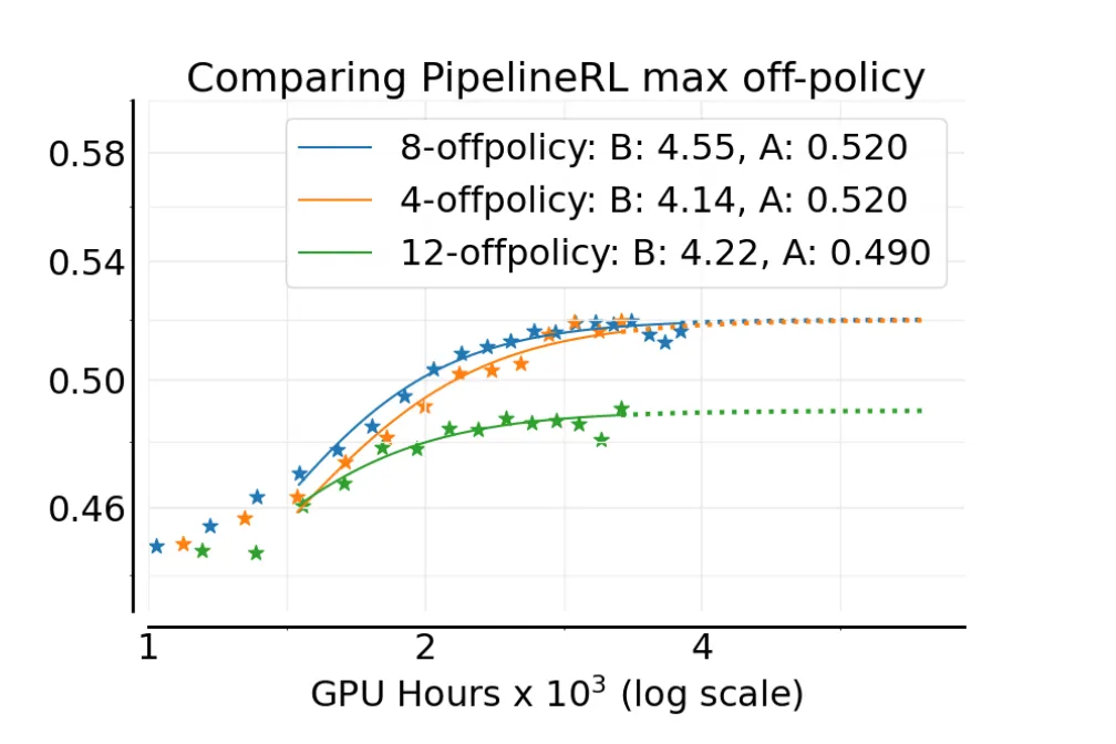
The influential PipelineRL paper from ServiceNow reframes the problem entirely. Instead of viewing RL as a tight, synchronous loop, it treats it as a distributed computing problem: a producer-consumer pipeline.
In this model, the system is decoupled into two main components:
- The actors (the data generators) are the producers. Their only job is to continuously run inference with their current version of the model policy, generating experiences and pushing them into a shared, centralized replay buffer.
- The learner (the trainer) is the consumer. It runs on its own schedule, constantly pulling batches of data from the replay buffer to perform its training updates.
After an update, the learner broadcasts its new, improved policy weights back out to the actors, who then seamlessly adopt them for future generations. Critically, the actors do not stop any of their existing chains of thought, but instead continue token generation on top of an effectively stale KV cache. Even though the cached key value tensors are from an “older” model, in practice the end product of the CoT is usually good enough.
This asynchronous, decoupled architecture smooths out the entire process. The actor never has to sit idle waiting for previous generations to finish before updating its weights; instead can always be generating new data. Likewise, the generators never have to stop and wait for a training step to complete. Each component can operate at its maximum possible speed, dramatically increasing overall hardware utilization.
4) Kimi's Hybrid Deployment / Engine Switching
While PipelineRL offers an elegant architectural solution, the team at Moonshot AI faced a problem of such massive scale that it required a different, more audacious approach. As detailed in their Kimi K2 paper, their model was so large that it required a minimum of 256 GPUs just to hold it in memory. The financial implication of allowing a 256-GPU cluster to sit idle, even for a few minutes, is, as we say in the business, “not good.”
Their solution, which they call Hybrid Deployment or "engine switching" is unusual. Instead of having separate clusters for training and inference, they use a single, massive cluster for both, dynamically reconfiguring its purpose on the fly. The process is as follows:
- First, the cluster is configured for training. The training engine, model weights, and massive optimizer states are loaded into the 256 GPUs' memory, and a single training step is performed.
- The main issue here is sharding. Each engine has a different sharding paradigm, and yet the inference engine must obtain updated parameters from the training engine nonetheless.
- To solve this, they created a Checkpoint Engine that is co-located on training nodes to manage these parameter states. Each checkpoint engine worker broadcasts all of its parameters to every other worker.
- Then, the inference workers just pick and choose the parameter chunks they need from this large broadcasted “stream” of data.
The authors note the obvious tradeoff of broadcasting this much data even when only a subset is needed for inference. But they believe it’s the right decision because it’s significantly simpler than alternatives, and the ability to fully decouple training and inference makes maintenance and testing way easier.
Conclusion and further reading
Like I mentioned earlier, maximizing generation efficiency during RL training is an area of active research without any clear best practices at the moment. Once can glean snippets and ideas from popular papers about scaling RL, but like the rest of the scaling RL “stack” there is significantly less consensus on these topics than for core pre-training for LLMs.
Additionally, many of the details and examples in this post are taken from Ai2’s RL setup; they released their state of the art completely open reasoning model, Olmo 3, last week, along with all of weights, training code, etc. (when I say completely open I mean it). You can read their technical breakdown here.
Sources and further reading
- Olmo 3 Technical Report
- Asynchronous RLHF: faster and more efficient off-policy RL for language models
- The Art of Scaling Reinforcement Learning Compute for LLMs
- PipelineRL: Faster On-policy Reinforcement Learning for Long Sequence Generation
- Kimi K1.5: Scaling Reinforcement Learning With LLMs
- Kimi K2: Open Agentic Intelligence